GANs —
Wasserstein GAN with MNIST (Part 6)
Brief theoretical introduction to Wasserstein GAN or WGANs and practical implementation using Python and Keras/TensorFlow in Jupyter Notebook.

In this article, you will find:
- Research paper,
- Definition, network design, and cost function, and
- Training WGANs with MNIST dataset using Python and Keras/TensorFlow in Jupyter Notebook.
Research Paper
Arjovsky, M., Chintala, S., & Bottou, L. (2017). Wasserstein GAN. ArXiv, abs/1701.07875.
Wasserstein GAN — WGAN
Wasserstein GAN (WGAN) proposes a new cost function using Wasserstein distance that has a smoother gradient everywhere.
This model is proposed to measure the difference between the data distributions of real and generated images.
This network is very similar to the Discriminator 𝐷 just without the sigmoid function and outputs a scalar score rather than a probability.
The Discriminator 𝐷 is renamed to Critic to reflect its new role.
Read more about GANs:
Network design

x is the real data and z is the latent space.
Cost function

Training WGANs
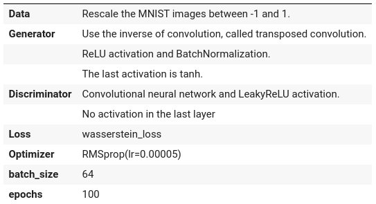
- Data: MNIST dataset
(X_train, y_train), (X_test, y_test) = mnist.load_data()2. Model:
- Generator
# Generator network
generator = Sequential()# FC
generator.add(Dense(7*7*512, input_shape=(latent_dim,), kernel_initializer=init))
# generator.add(ReLU())
generator.add(Reshape((7, 7, 512)))

# Conv 1 and Con 2
...

# Output
generator.add(Conv2DTranspose(1, kernel_size=3, strides=2, padding='same', activation='tanh'))
- Critic
# Critic network
critic = Sequential()

# Conv 1
critic.add(Conv2D(64, kernel_size=3, strides=2, padding='same', input_shape=(img_shape)))
critic.add(LeakyReLU(0.2))

# Conv 2, Conv 3 and Conv 4
...# FC
critic.add(Flatten())

# Output
critic.add(Dense(1))
3. Compile
# Wasserstein objective
def wasserstein_loss(y_true, y_pred):
    return K.mean(y_true * y_pred)n_critic = 5
clip_value = 0.01
optimizer = RMSprop(lr=0.00005)

critic.compile(optimizer=optimizer, loss=wasserstein_loss, metrics=['accuracy'])critic.trainable = False  # The generator takes noise as input and generated imgs
z = Input(shape=(latent_dim,))
img = generator(z)  # The critic takes generated images as input and determines validity valid = critic(img)  # The combined model (critic and generative)
c_g = Model(inputs=z, outputs=valid, name='wgan')  c_g.compile(optimizer=optimizer, loss=wasserstein_loss, metrics=['accuracy'])s
4. Fit
for _ in range(n_critic):

    # Train Discriminator weights
    critic.trainable = True

    # Real samples
    X_batch = X_train[i*batch_size:(i+1)*batch_size]
    d_loss_real = critic.train_on_batch(x=X_batch, y=real)

    # Fake Samples
    z = np.random.normal(loc=0, scale=1, size=(batch_size, latent_dim))
    X_fake = generator.predict(z)
    d_loss_fake = critic.train_on_batch(x=X_fake, y=fake)

    # Discriminator loss
    d_loss_batch = 0.5 * (d_loss_real[0] + d_loss_fake[0])

    # Clip critic weights
    for l in critic.layers:
        weights = l.get_weights()
        weights = [np.clip(w, -clip_value, clip_value) for w in weights]
        l.set_weights(weights)

    # Train Generator weights
    critic.trainable = False
    g_loss_batch = c_g.train_on_batch(x=z, y=real)
5. Evaluate
# plotting the metrics
plt.plot(d_loss)
plt.plot(d_g_loss)
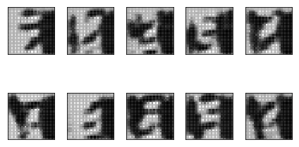
plt.show()WGANs — MNIST results
Train summary
Github repository
Look the complete training WGAN with MNIST dataset, using Python and Keras/TensorFlow in Jupyter Notebook.
For those looking for all the articles in our GANs series. Here is the link.